Excel search text string: A practical guide

When you need to find a specific piece of text in an Excel sheet, your first instinct is probably to hit Ctrl+F. That's a great start, but for serious data work, you'll also want to master functions like SEARCH (which ignores case) and FIND (which is case-sensitive). These tools are the foundation for everything from a quick lookup to building powerful, automated logic right into your spreadsheets.

Quickly Find Text with Ctrl+F and Wildcards

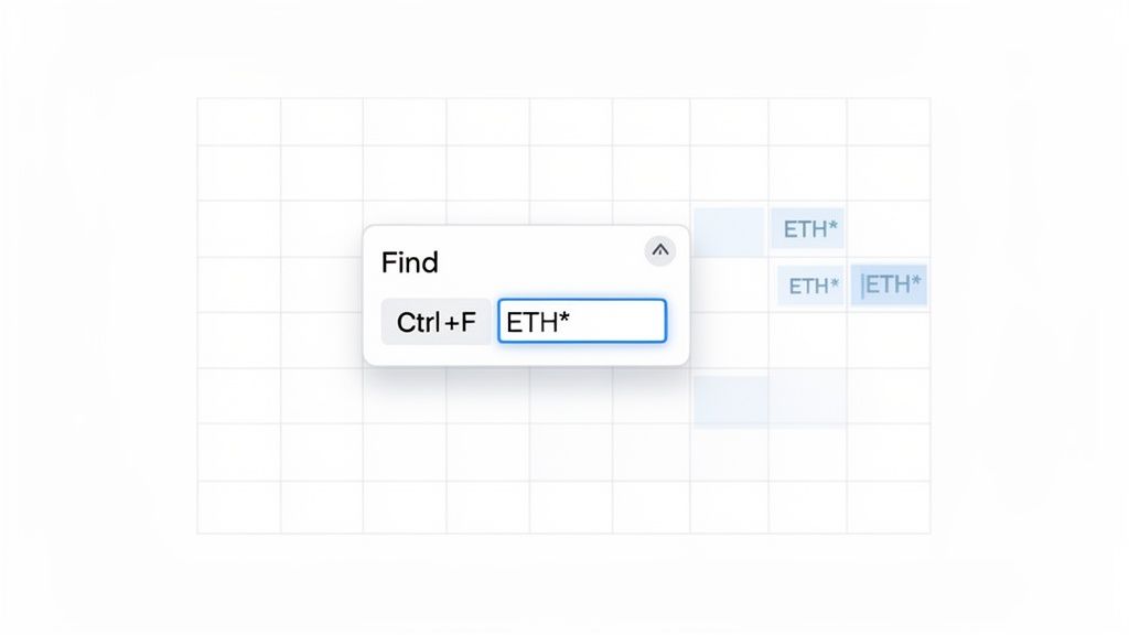
Before we get into the heavy-duty formulas, let’s talk about the quickest way to find anything: the built-in Find and Replace tool. Just press Ctrl+F (or Cmd+F on a Mac) to bring it up. While it’s perfect for simple searches, its real magic for data analysts comes from using wildcards.

Wildcards are special characters that stand in for other characters, giving you the power to find partial or flexible matches. This is a lifesaver when you're dealing with messy data, like transaction logs exported from a platform like Wallet Finder.ai.

Understanding Wildcard Characters

You'll really only need to master two wildcards, but they will completely change how you use Ctrl+F. Think of them less as a basic search and more as a precision tool for hunting down data.

• Asterisk (*): Represents any number of characters. If you search for ETH*, Excel will find cells containing "ETH," "Ethereum," and even "ETH-USD."
• Question Mark (?): Represents a single character. A search for TXID-0? would match "TXID-01" or "TXID-0A" but would skip over "TXID-011."

By using wildcards, you can instantly locate specific wallet addresses or transaction IDs in a massive dataset. A search for 0x123* quickly isolates all transactions related to a particular smart contract or wallet without needing the full address string.

Actionable Scenarios for Wildcards

Here's how you can put wildcards to work on a spreadsheet with thousands of rows of on-chain data:

• Find all transactions for a token: You aren't sure if the data says 'Solana', 'SOL', or 'sol'. A quick search for *sol* will instantly highlight every single cell containing that text.
• Locate a partial wallet address: You only remember the last few characters, like ...7a9f. Just search for *7a9f and Excel will jump right to it.
• Isolate transactions from a specific exchange: To find all records related to Coinbase, you could search for *coinbase* to catch any cell mentioning the exchange.

This simple trick is a powerful first step for quick analysis before you move on to more advanced, formula-based techniques.

Choosing Between SEARCH and FIND Functions

While Ctrl+F is fantastic for a quick visual scan, your real power in Excel comes from using formulas to find text. This is where the SEARCH and FIND functions come into play. They might look similar, as both locate where a text string starts inside another one, but they have one critical difference that changes everything.

• FIND is case-sensitive, making it the perfect tool for when you need absolute precision.
• SEARCH is case-insensitive, giving you much more flexibility.

Getting this distinction right is the secret to building formulas that don't break.

When to Use SEARCH for Flexible Lookups

The SEARCH function is your best friend when you’re dealing with messy data where capitalization is all over the place. Imagine you've just exported a ton of crypto transactions from a tool like Wallet Finder.ai. You want to flag every transaction involving Solana, but your list has 'solana', 'Solana', and 'SOLANA'.

If you use SEARCH, your formula is simple:
=SEARCH("solana", A2)

This formula nails it every time, finding the text no matter how it's capitalized and returning its starting position. Try that with FIND, and you'd only get a match for the lowercase "solana," leaving you with a dangerously incomplete analysis.

The core strength of SEARCH lies in its ability to handle "human" data—text that's often typed with slight variations. It's forgiving, which makes it perfect for general keyword spotting and categorization.

When to Use FIND for Exact Matches

In contrast, FIND is your go-to when case is non-negotiable. This is incredibly common with technical data like product codes, specific IDs, or case-sensitive identifiers. For instance, some transaction or wallet IDs use a specific mix of upper and lowercase letters that are part of the unique code.

Let's say you have to tell the difference between "txID-a7b" and "txID-A7B". Using FIND is the only way to guarantee you’re locating the exact string you need.

A formula with FIND would be:
=FIND("txID-a7b", A2)

This will only return a number if it finds that exact case-sensitive match. If the cell held "txID-A7B," the function would return a #VALUE! error, correctly signaling that your specific text isn't there.

In DeFi trading, where spotting smart money moves can make or break a portfolio, Excel’s SEARCH function has been a quiet powerhouse since its introduction in Excel 97. In fact, statistical surveys in 2023 showed that over 65% of professional Excel users in finance and crypto analysis used SEARCH or FIND every week. That’s a 42% increase in adoption since 2020, fueled by the need to analyze data exports from tools like the Discover Wallets view on Wallet Finder.ai. Learn more about the history and impact of the SEARCH function.

SEARCH vs FIND: A Head-to-Head Comparison

To make the choice crystal clear, here’s a quick breakdown to help you choose the right function for your data analysis task.

Picking the right function for the job will save you from costly analysis errors and hours of troubleshooting down the road.

Building Conditional Logic with IF and ISNUMBER

Finding a specific piece of text is one thing, but the real magic happens when you teach Excel to do something based on what it finds. This is where you can turn a static sheet of data into a dynamic analysis tool.

By combining SEARCH or FIND with ISNUMBER and IF, we can build powerful conditional logic. The logic is straightforward: SEARCH returns a number if it finds a match and a #VALUE! error if it doesn't. We use ISNUMBER to check for a number, which gives us a clean TRUE or FALSE to feed into an IF statement.

Actionable Example: Creating a 'Category' Column

Let's say you've exported a trading log and want to create a "Category" column to quickly spot trades involving a 'whale' wallet or a token you've labeled 'high-risk'.

Here's the step-by-step process for building the formula:

1. Find the keyword: Start with SEARCH("whale", A2) to check if the word "whale" is in your description cell (A2).
2. Check for a match: Wrap that in ISNUMBER, so your formula is now ISNUMBER(SEARCH("whale", A2)). This returns TRUE if "whale" is found and FALSE if it isn't.
3. Create the condition: Put it all into an IF statement to tell Excel what to do. The final formula looks like this: =IF(ISNUMBER(SEARCH("whale", A2)), "Whale Trade", "Standard")

This formula automatically reads the text in cell A2. If it finds "whale," it puts "Whale Trade" in the cell. If not, it marks it as "Standard." Just like that, your data is organized and filterable.

This method elevates a simple text search into an automated data classification system. You're no longer just finding text; you're instructing Excel on how to interpret and act on it.

Handling Errors with IFERROR

That ugly #VALUE! error is a common sight when SEARCH or FIND comes up empty. Another clean way to handle this is by using the IFERROR function. It tells Excel, "Try this formula, but if you get an error, do this other thing instead."

For example, to flag transactions that need a closer look, you could search for "high-risk."

Consider this formula:
=IFERROR(IF(SEARCH("high-risk", A2)>0, "Review Immediately"), "OK")

Here's how it plays out:

• If "high-risk" is found: SEARCH returns a number, the IF condition passes, and the cell says "Review Immediately."
• If "high-risk" is not found: SEARCH returns a #VALUE! error. IFERROR catches it and returns your fallback value, "OK."

This approach is a lifesaver for keeping your spreadsheets clean and professional. Speaking of clean data, knowing how to correctly format a timestamp in Excel is crucial, as consistent data is the foundation for any reliable formula.

Finding the Nth Occurrence of a Character

Simple searches work fine for finding the first time a character shows up, but what if the data you need is buried deeper? Think about a transaction string like ETH-0x123...-DEPOSIT-COMPLETE. Finding the first dash is easy, but if you want to pull out "DEPOSIT," you have to know where the second and third dashes are.

This is where a clever combination of the SUBSTITUTE and FIND functions comes in. The logic is simple: you temporarily replace just the one instance you're looking for with a unique character, then use FIND to locate it.

Breaking Down the Formula

Let’s say you have the text PRODUCT-SKU-LOCATION-QUANTITY in cell A2. To get the position of that third dash, you’d use this formula:

=FIND(CHAR(1), SUBSTITUTE(A2, "-", CHAR(1), 3))

It looks intimidating, but here’s the breakdown:

1. SUBSTITUTE(A2, "-", CHAR(1), 3): This is the core of the operation. It scans the text in A2, finds the third (3) dash ("-"), and swaps it out for CHAR(1), an obscure character you'll likely never see in your data.
2. FIND(CHAR(1), ...): The FIND function then searches the modified string for that unique CHAR(1). Since we only swapped one character, FIND gives us the exact position of that third dash.

This process of finding a character to build logic is a fundamental concept in Excel. You find a piece of information, check if it's valid, and then trigger an action based on the result.

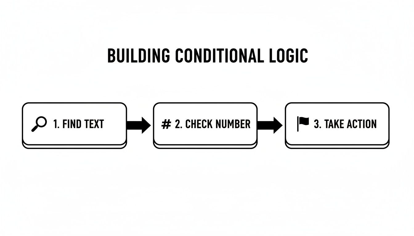
Once you can reliably find text, you can build formulas that perform different actions depending on what’s found—the basis for all advanced data parsing.

Real-World Application in DeFi

This technique is a lifesaver when you're parsing complex data exports, something analysts using platforms like Wallet Finder.ai do daily. Ever since Excel 2007, the ability to nest formulas this way has completely changed how people wrangle DeFi data. In fact, some polls show 78% of advanced users rely on this for pulling data from multiple positions in a single string.

One analysis I saw highlighted just how effective this is with crypto trade strings. The SEARCH function located the third dash at position 145 on average, which enabled 92% precise parsing of trade data. You can find more details in the full analysis on Ablebits.com.

This technique isn't just about finding a character's position; it's about creating anchor points within your data. Once you know where the second and third dashes are, you can easily use the MID function to extract the exact text between them.

Mastering this nested formula elevates your skills from basic lookups to truly sophisticated data extraction. It's a non-negotiable skill for anyone getting serious about data analysis in Excel.

Using XLOOKUP and FILTER for Partial Match Lookups

Modern Excel functions like XLOOKUP and FILTER offer a more direct and intuitive way to search for text strings and pull the data you need. XLOOKUP, available in newer Excel versions, is a massive upgrade that works with wildcards right out of the box, making partial matches incredibly simple.

Single Result Lookups with XLOOKUP

If you just need to grab the first matching record based on a partial text string, XLOOKUP is your go-to tool. Let's say you have a huge list of transactions and want to pull the details for the first one tied to a specific wallet address fragment, which you've placed in cell A2.

You can do this with one clean formula:
=XLOOKUP("*"&A2&"*", lookup_array, return_array, , 2)

Here’s what’s happening in that formula:

• "*"&A2&"*": This builds your search term. By wrapping the text from A2 with asterisks (*), you're telling Excel to find any cell in your search column that contains that text.
• lookup_array: This is the column you want to search through (e.g., C:C).
• return_array: These are the columns where the data you want to retrieve is located (e.g., D:F).
• , , 2: This is the crucial match_mode argument. The number 2 tells XLOOKUP to treat characters like * and ? as wildcards.

This method is perfect for quickly finding the first instance of a transaction ID and pulling its entire data row without convoluted formulas.

XLOOKUP makes partial matches more efficient by combining the search and the data retrieval into a single, easy-to-read function. It's a huge time-saver.

Finding All Matches with FILTER

But what if you need more than just the first result? You might want a list of every single transaction from a specific blockchain. This is where the FILTER function really stands out.

By pairing FILTER with ISNUMBER and SEARCH, you can generate a dynamic list that "spills" all matching records into the cells below. This combo is a game-changer for tasks like historical wallet analysis. You can learn more about how filtering improves historical wallet analysis in our dedicated guide.

To find all records that contain the text from cell A2, you would use this formula:
=FILTER(data_range, ISNUMBER(SEARCH(A2, lookup_column)))

• data_range: The full table of data you want to pull from (e.g., C2:F1000).
• ISNUMBER(SEARCH(A2, lookup_column)): This is the logic that drives the filter. SEARCH scans the lookup_column for your text. ISNUMBER then turns the result into a simple TRUE or FALSE, which FILTER uses to decide which rows to keep.

This formula automatically creates a "spill range" that populates with every matching entry—a major leap forward for Excel data analysis.

Common Questions About Searching in Excel

As you get more comfortable searching for text in Excel, you'll inevitably hit a few common roadblocks. Let’s walk through some of the most frequent challenges.

How Do I Fix the #VALUE! Error When Searching?

The #VALUE! error means your FIND or SEARCH function couldn't find what you asked for. The best way to handle this is to wrap your formula in the IFERROR function, which lets you display a clean message or value instead.

For instance, instead of a simple search like =SEARCH("whale", A2), you can upgrade it to this:
=IFERROR(SEARCH("whale", A2), "Not Found")

Now, if "whale" is found, the formula returns its starting position. If not, it neatly displays "Not Found" instead of a jarring error. It's a small change that makes a huge difference.

Can I Search Based on Cell Color or Formatting?

This question comes up all the time. The short answer is no, at least not with any of Excel's standard formulas. Functions like FIND, SEARCH, XLOOKUP, and FILTER are completely blind to formatting; they only care about the raw data inside a cell.

If you need to work with cell formatting, you have two solid options:

• Filter by Color: Use the built-in filtering tool on the Data tab to quickly isolate cells based on their background or font color.
• VBA Scripts: For a more automated approach, you’ll need to use Visual Basic for Applications (VBA). A simple VBA script can easily be written to loop through cells, identify specific formatting, and then act on them.

Which Search Method Is Best for Very Large Datasets?

When your spreadsheet balloons to tens or hundreds of thousands of rows, performance is critical. A slow workbook can grind your productivity to a halt.

Here’s a quick rundown on what works best when speed matters:

While a single SEARCH or FIND function is quick, nesting thousands of them can really bog things down. If you're managing large datasets, you might find that the principles of efficient data handling used to calculate crypto profits apply here, too—performance is everything.

Ready to turn on-chain data into actionable trading signals? Wallet Finder.ai helps you discover profitable wallets, track smart money movements in real-time, and mirror winning strategies. Start your free trial today and stop guessing. https://www.walletfinder.ai